Tutorial 15: Joint Seismic-Electrical Inversion (Sleipner)#
Note
This tutorial is available as a Python script examples/15_sleipner_joint_inv.py and an interactive Jupyter notebook examples/notebooks/15_sleipner_joint_inv.ipynb.
Jointly invert seismic and resistivity data to recover porosity and CO₂ saturation for the Sleipner CO₂ storage site in the Norwegian Sea.
What You Will Learn#
Combine multiple physics (seismic + resistivity) in a single objective
Use rock physics to link seismic velocities and electrical resistivity
Build a 3D convolutional decoder for network parameterization
Run joint inversion with
Inverter.create_network()Interpret CO₂ saturation from inverted properties
Key Concepts#
Joint inversion exploits complementary sensitivities of different geophysical methods. Seismic data are sensitive to velocity contrasts while resistivity data (via Archie’s law) are sensitive to fluid saturation changes caused by CO₂ replacing brine.
Network parameterization uses a 3D convolutional decoder as the model representation, providing implicit spatial regularization and enabling joint inversion of multiple properties from a shared latent space.
The Sleipner CO₂ storage project has injected CO₂ into the Utsira Sand since 1996, making it one of the longest-running industrial carbon storage operations. Time-lapse seismic monitoring has tracked the growing CO₂ plume, and complementary resistivity data provide additional sensitivity to saturation changes. This tutorial combines both data types in a single objective function, using rock-physics relationships (Soft Sand, Gassmann fluid substitution, and Archie’s law) to link the shared model parameters – porosity and CO₂ saturation – to the two sets of observations.
Code#
from geobrain.physics.wave import Shuey, RickerWavelet, create_conv_matrix
from geobrain.physics.rock import SoftSand, Gassmann, ArchieResistivity
from geobrain.optim import Inverter

inverter = Inverter.create_network(
    decoder=decoder,
    forward_fn=joint_forward,
    observed=d_obs,
)

result = inverter.run(max_epochs=1000, lr=0.001)
Results#
The observed data comprise seismic traces and resistivity measurements, both of which carry information about the subsurface porosity and CO₂ saturation distribution.
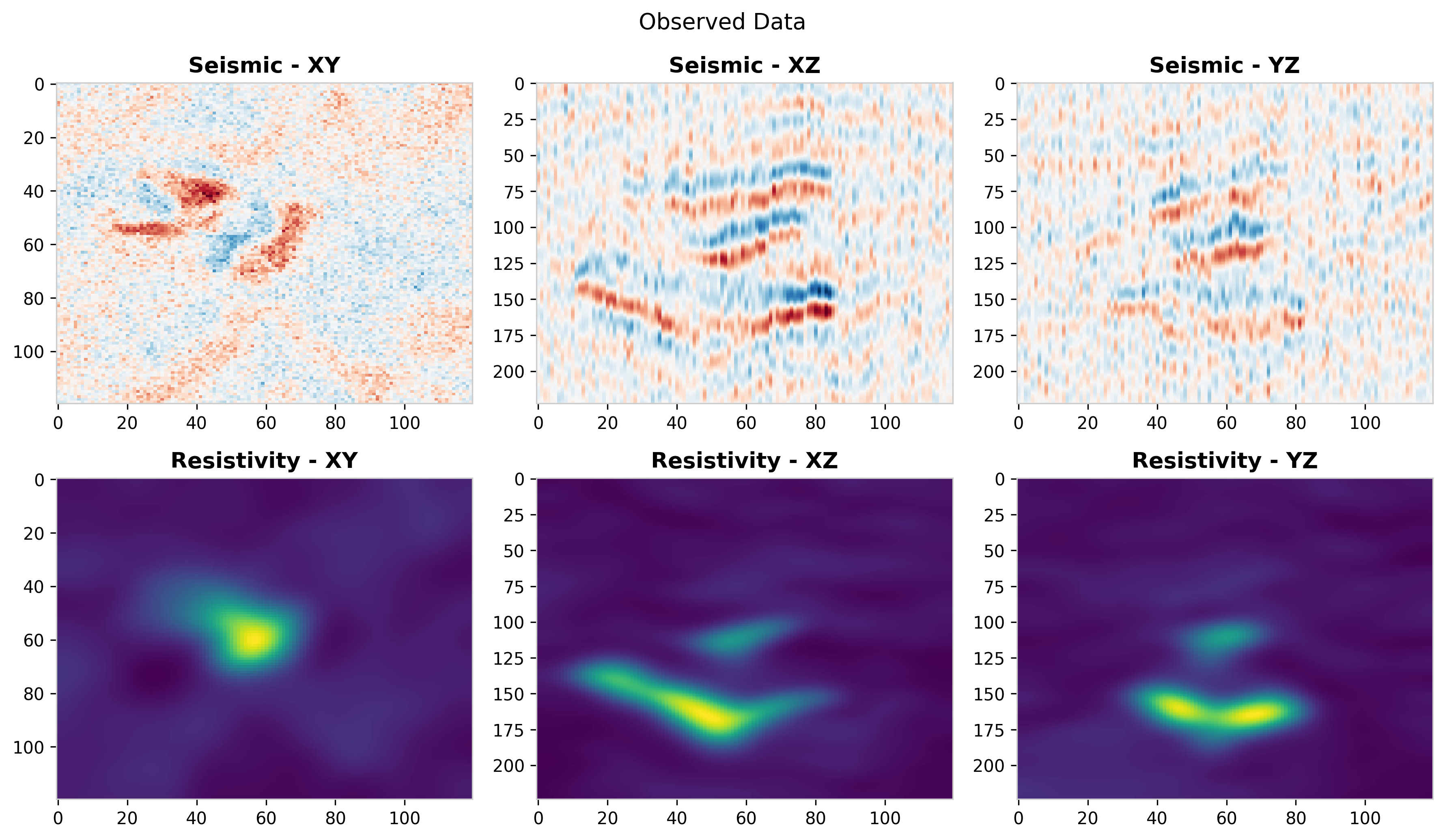
Fig. 76 Observed seismic and resistivity data.#
The joint inversion recovers porosity and CO₂ saturation models that are consistent with both data types simultaneously. The network parameterization enforces spatial smoothness and couples the two properties through a shared latent code.
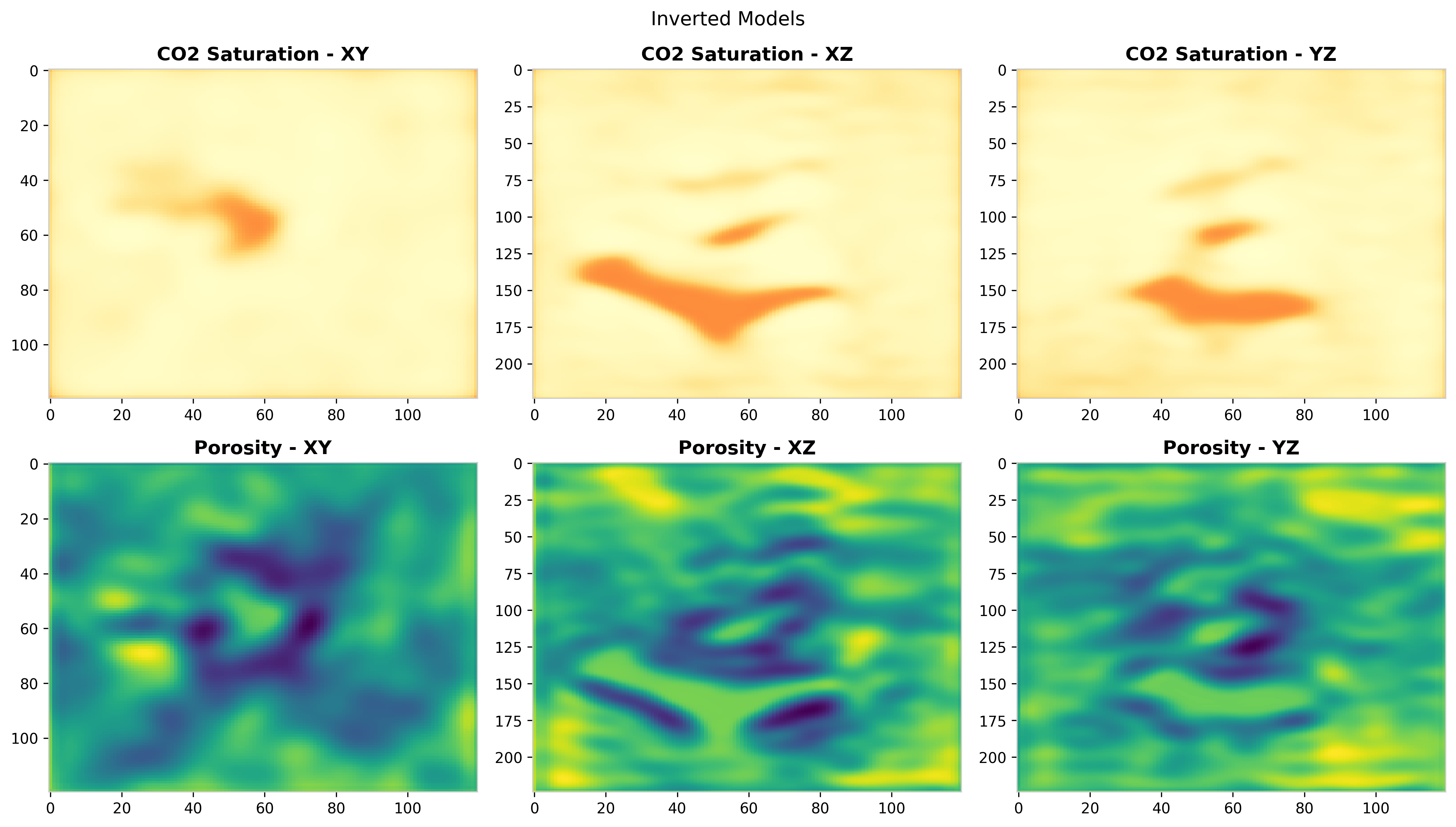
Fig. 77 Inverted porosity and CO2 saturation models.#
The convergence curve shows steady reduction of the combined objective function over iterations, confirming that the optimizer successfully minimizes the misfit to both seismic and resistivity data.
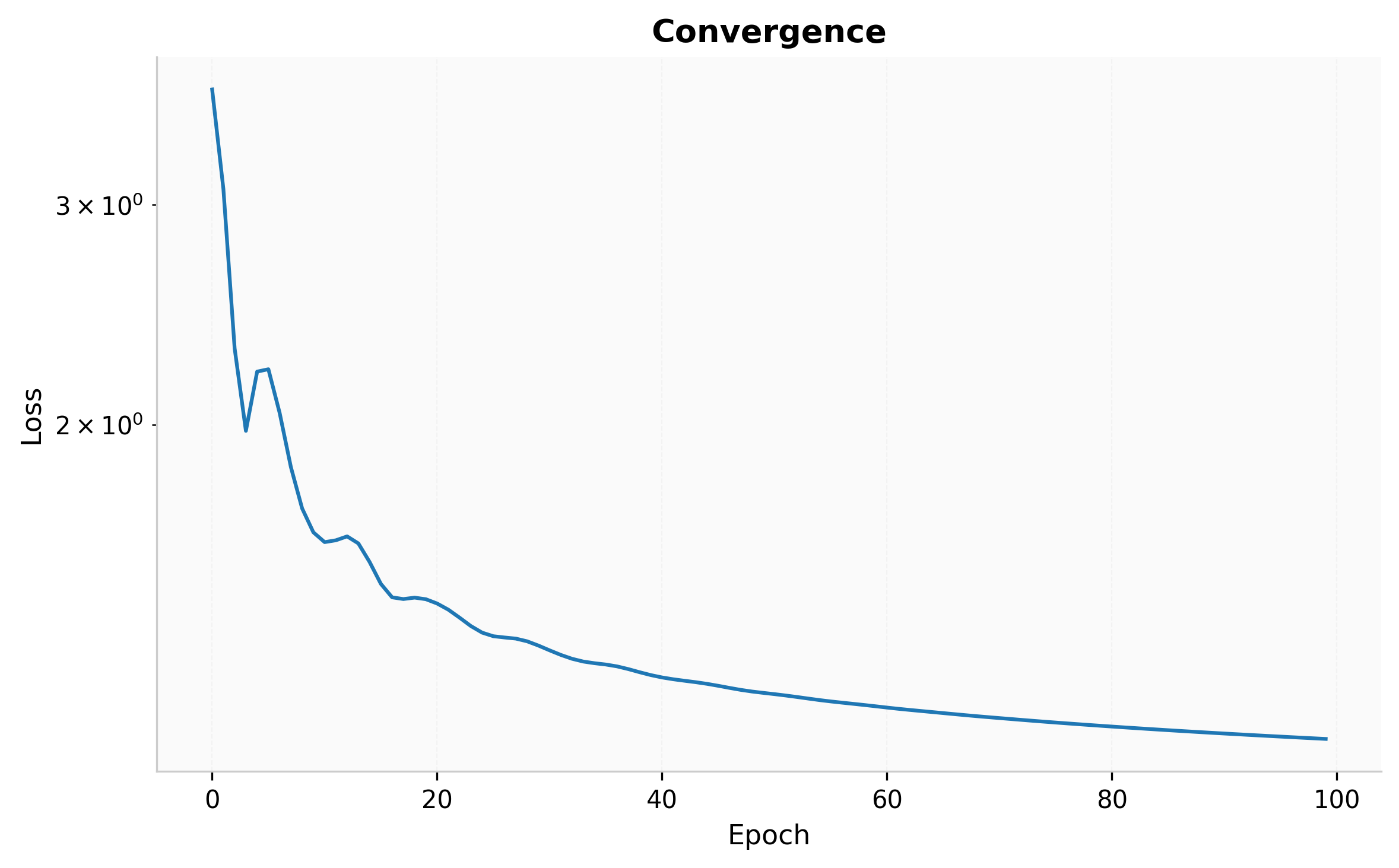
Fig. 78 Joint inversion convergence curve.#