Bayesian inference (geobrain.bayes)

The second door on an InverseProblem. Same object, same objective. The difference is that a sampler explores -log posterior instead of descending it.

# sketch: runnable version in the quick start
posterior = problem.as_posterior(transforms={"vp": PositiveTransform()})
draws = posterior.sample("nuts", params=start, n_iters=300, ctx=ctx, warmup=100)

Piece	What is there
Samplers	HMC, NUTS, LangevinDynamics, SVGD, one string apart
Transforms	PositiveTransform, IntervalTransform, IdentityTransform, InvertibleTransform
Distributions	Gaussian, GaussianMixture, Distribution
Chains	run_chains, ChainConfig, InferenceResult, RunAccounting
Diagnostics	split_rhat, ess, summarize

Bounds are transforms, not clipping

PositiveTransform and IntervalTransform are changes of variable: the sampler works in an unbounded space and the model comes back inside its physical range by construction, with the Jacobian accounted for. Clipping a proposal instead would break detailed balance and quietly bias the posterior toward the bound.

Read the diagnostics before the answer

Two numbers decide whether the run means anything

R-hat compares the variance between chains to the variance within them. Above about 1.01, the chains have not found the same distribution and the posterior you are looking at is an artefact of where they started.

ESS is how many independent draws your correlated ones are worth. A thousand samples with an ESS of 40 is forty samples with extra steps, so quote nothing below about 100.

summarize reports both per parameter. The Bayesian workflow example draws them and says what to do when they are bad.

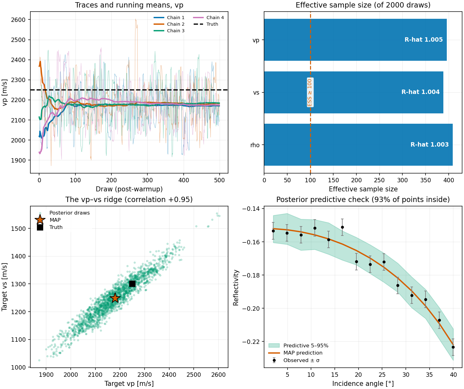
Chains, R-hat, effective sample size and a posterior predictive check, in the order you should look at them. From examples/01_architecture/06_bayesian_workflow.py.

Why bother

A deterministic inversion returns one model. The posterior returns the set of models the data have not ruled out, and the width of that set, propagated through whatever comes next, is the difference between an answer and an answer you can act on. Because the rock physics is in the same graph, a posterior on porosity propagates into a posterior on velocity for free.

See also

• examples/01_architecture/06_bayesian_workflow.py: chains, R-hat, ESS and the posterior predictive check.

• examples/00_showcase/04_deterministic_bayes_unified.py: both doors on one rock-physics AVO problem, with the MAP loss checked against -problem.log_posterior to the digit.