Flow Simulation (geobrain.physics.flow)#
The flow module provides differentiable reservoir simulation for single- and multi-phase fluid flow through porous media.
Overview#
The flow simulator solves the pressure and saturation equations on a structured grid, supporting:
Single-phase and two-phase (oil-water) flow
Well injection and production with rate or BHP control
PVT (pressure-volume-temperature) properties
Relative permeability models (Corey or tabular)
Differentiable solver for gradient-based history matching
Step-by-step simulation with dynamic well control
Basic Usage#
from geobrain.physics.flow import (
    ReservoirModel, FlowPropagator, Well, compute_well_index
)

# Create reservoir model
model = ReservoirModel(nx=50, ny=50, nz=1)
model.set_grid(dx=10.0, dy=10.0, dz=5.0)
model.set_rock(perm=perm_field, poro=poro_field)
model.set_pvt(pvdo=pvdo_table, pvtw=pvtw_table)
model.set_relperm(corey={'swc': 0.2, 'sor': 0.2, 'nw': 2.0, 'no': 2.0})
model.initialize(po=initial_pressure, sw=initial_saturation)

# Create wells
wi = compute_well_index(kx=100, ky=100, dx=10, dy=10, dz=5, rw=0.5)

inj = Well('INJ1', well_type='INJ')
inj.add_perforation(cell_idx=0, wi=wi)
inj.set_control('RATE', target=-500.0, phase='WATER')
model.add_well(inj)

prod = Well('PROD1', well_type='PROD')
prod.add_perforation(cell_idx=2499, wi=wi)
prod.set_control('BHP', target=200.0)
model.add_well(prod)

# Run simulation
propagator = FlowPropagator(model)
result = propagator(t_end=365.0, dt_init=1.0, dt_max=10.0)

# Access results
pressure = result.pressure       # List of tensors per timestep
saturation = result.saturation   # List of tensors per timestep
well_data = result.well_data     # Well histories by name
Fig. 21 Two-phase oil-water flow simulation: pressure and saturation evolution.#
Dynamic Well Control#
Wells can be added, shut in, or have rates changed mid-simulation using step-by-step mode:
propagator = FlowPropagator(model)

# Phase 1: initial production
result1 = propagator(t_end=180.0, dt_init=1.0)

# Phase 2: change well control
prod.set_control('RATE', target=300.0, phase='LIQ')
result2 = propagator(t_end=365.0, dt_init=1.0)
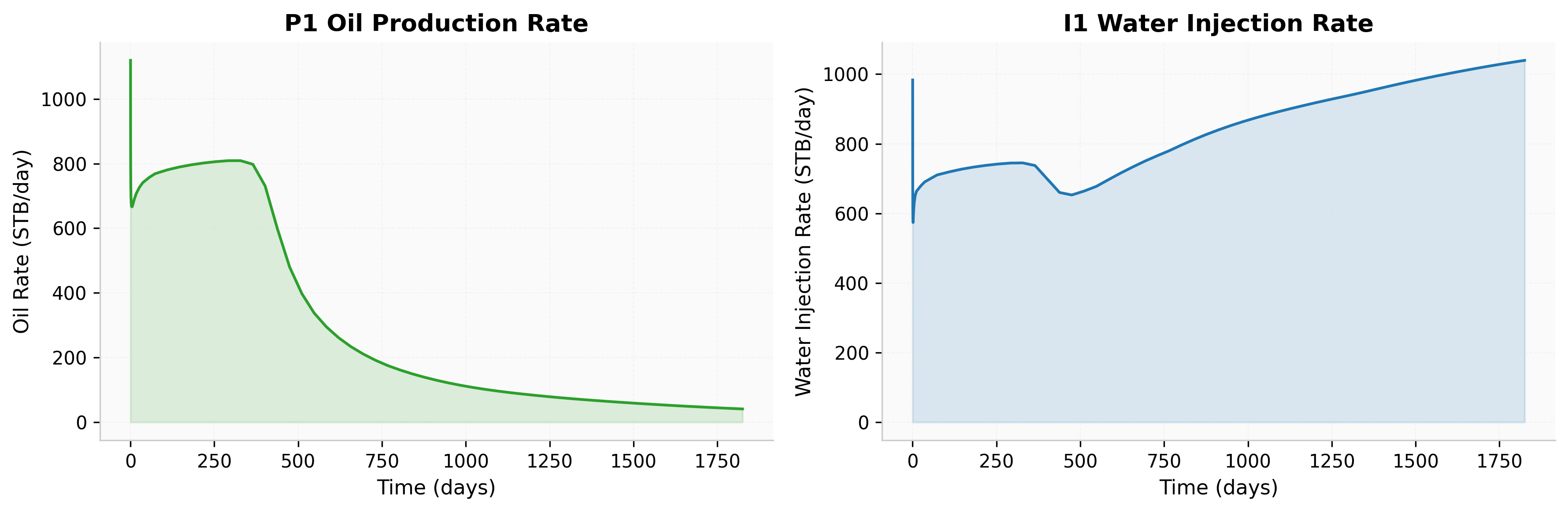
Fig. 22 Production curves: oil rate, water rate, and water cut.#
Differentiability#
The flow solver supports automatic differentiation for history matching:
import torch

# Permeability as a differentiable parameter
perm = torch.tensor(perm_field, requires_grad=True)
model.set_rock(perm=perm, poro=poro_field)

propagator = FlowPropagator(model)
result = propagator(t_end=100.0, dt_init=1.0)
loss = torch.nn.functional.mse_loss(result.pressure[-1], observed_pressure)
loss.backward()  # Gradient of loss w.r.t. permeability
Well Index#
The Peaceman formula computes the well-reservoir coupling coefficient:
from geobrain.physics.flow import compute_well_index

wi = compute_well_index(
    kx=100,    # X-permeability (md)
    ky=100,    # Y-permeability (md)
    dx=100,    # Cell size x (ft)
    dy=100,    # Cell size y (ft)
    dz=20,     # Cell size z (ft)
    rw=0.5,    # Wellbore radius (ft)
    skin=0.0,  # Skin factor
)
Solver#
The implicit Newton solver handles nonlinear pressure-saturation coupling:
NewtonSolver: Fully implicit solver with automatic Jacobian
TimeStepScheduler: Adaptive time stepping based on convergence