Tutorial 10: Fluid Flow Simulation#
Note
This tutorial is available as a Python script examples/10_flow_simulation.py and an interactive Jupyter notebook examples/notebooks/10_flow_simulation.ipynb.
Simulate oil-water two-phase fluid flow through porous media using GeoBrain’s differentiable reservoir simulator.
What You Will Learn#
Set up a reservoir model with
ReservoirModelConfigure grid, rock properties, PVT data, and relative permeability
Add production and injection wells
Run flow simulation with
FlowPropagatorVisualize production curves and pressure/saturation maps
Key Concepts#
Two-phase flow simulation solves the coupled pressure and saturation equations on a reservoir grid. GeoBrain’s flow module is fully differentiable, enabling gradient-based history matching and optimization of well placement or injection strategy.
Water is injected through an injector well to maintain reservoir pressure and displace oil toward the producer. The simulator solves pressure and transport equations at each time step, updating the saturation front as it advances through the heterogeneous permeability field. Production curves record the oil rate, water rate, and water cut at the producer over time.
Code#
from geobrain.physics.flow import ReservoirModel, FlowPropagator, Well

model = ReservoirModel(
    grid=grid_config,
    rock=rock_props,
    pvt=pvt_data,
)

model.add_well(Well(name='INJ1', type='injector', ...))
model.add_well(Well(name='PROD1', type='producer', ...))

propagator = FlowPropagator(model)
result = propagator.run(n_steps=100, dt=1.0)
Results#
The pressure and saturation fields evolve as injected water displaces oil toward the production well. The maps below show snapshots at key time steps.
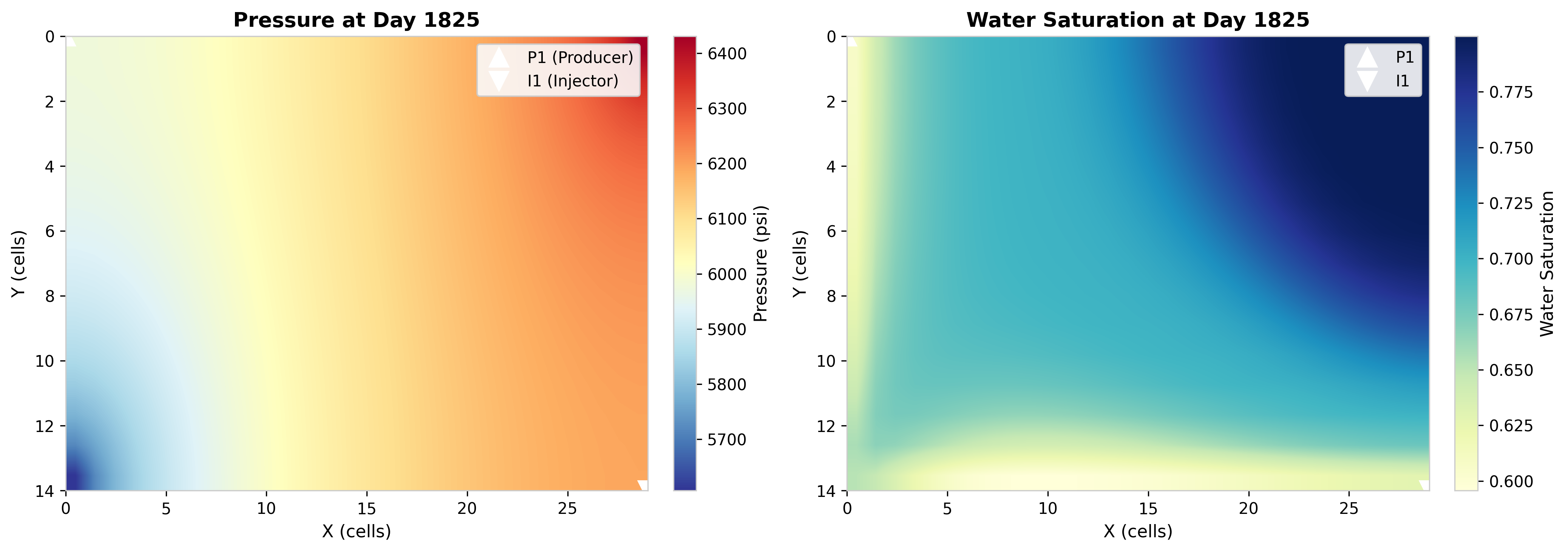
Fig. 60 Pressure and saturation maps at key time steps.#
Production curves capture the time history of oil rate, water rate, and water cut at the producer. Water breakthrough is visible as the oil rate declines and the water cut rises sharply.
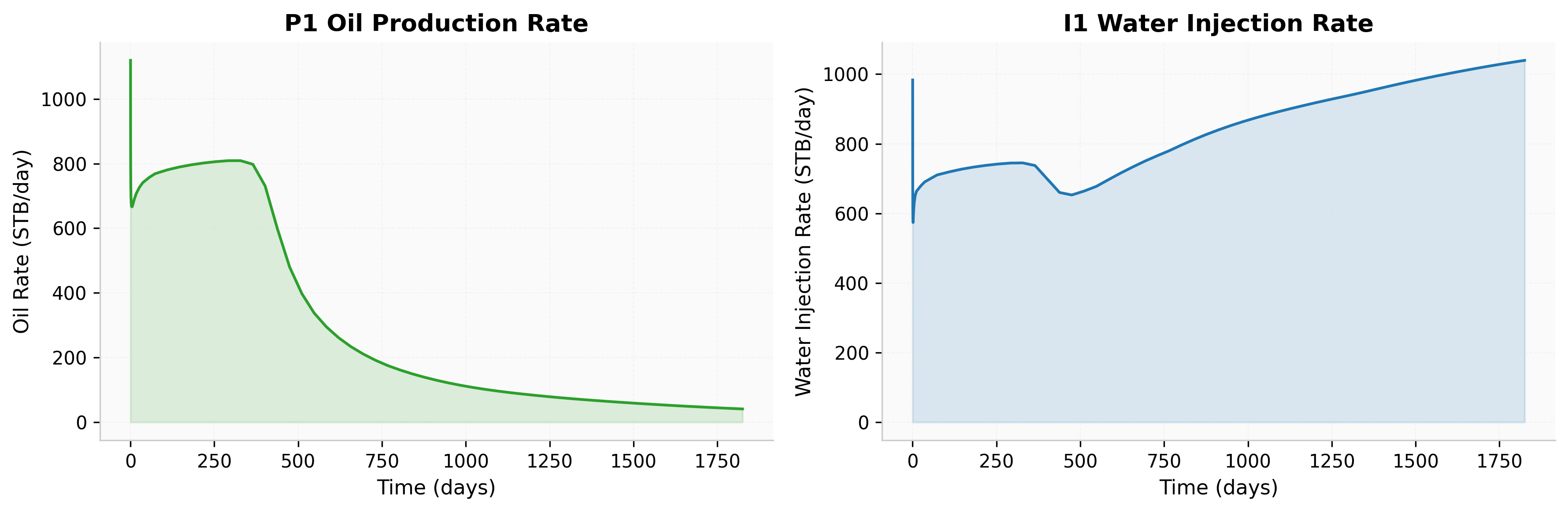
Fig. 61 Production curves: oil rate, water rate, and water cut.#
The following figure illustrates the full reservoir state evolution, tracking how the saturation front progresses through the domain at selected time steps.
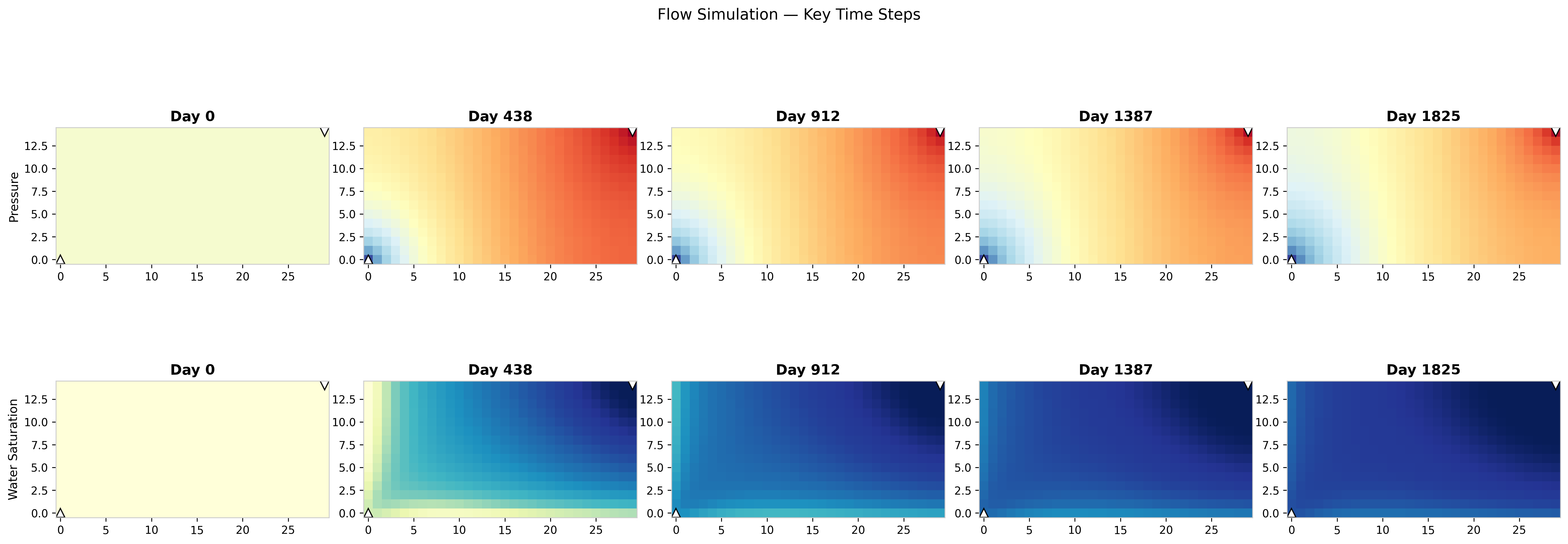
Fig. 62 Reservoir state evolution at key time steps.#