Tutorial 11: Dynamic Well Modeling#
Note
This tutorial is available as a Python script examples/11_flow_dynamic_wells.py and an interactive Jupyter notebook examples/notebooks/11_flow_dynamic_wells.ipynb.
Run step-by-step flow simulations with dynamic well control: add new wells, shut in existing wells, and change injection rates during the simulation.
What You Will Learn#
Configure wells with time-varying schedules (rates and BHP)
Run step-by-step simulation with
FlowPropagatorAdd and shut in wells mid-simulation
Monitor production profiles over time
Visualize time-lapse pressure and saturation maps
Key Concepts#
Dynamic well control allows modifying the well configuration between simulation time steps. This is essential for modeling real-world scenarios such as infill drilling, water injection optimization, and well shut-in for maintenance.
This tutorial demonstrates three simulation modes. First, a full simulation runs all time steps in a single call to establish a baseline. Second, a step-by-step simulation advances the same model one time step at a time, giving identical results while allowing inspection at arbitrary intermediate times. Third, dynamic well operations modify the well schedule mid-simulation – shutting in a producer and opening a new one – to show how the reservoir response changes under different management strategies.
Code#
from geobrain.physics.flow import ReservoirModel, FlowPropagator, Well

propagator = FlowPropagator(model)

# Step-by-step with dynamic control
for step in range(n_steps):
    if step == 50:
        model.shut_well('PROD1')
        model.add_well(Well(name='PROD2', ...))
    propagator.step(dt=1.0)
Results#
The full simulation runs all time steps at once, producing production curves and state maps that serve as the reference baseline for subsequent experiments.
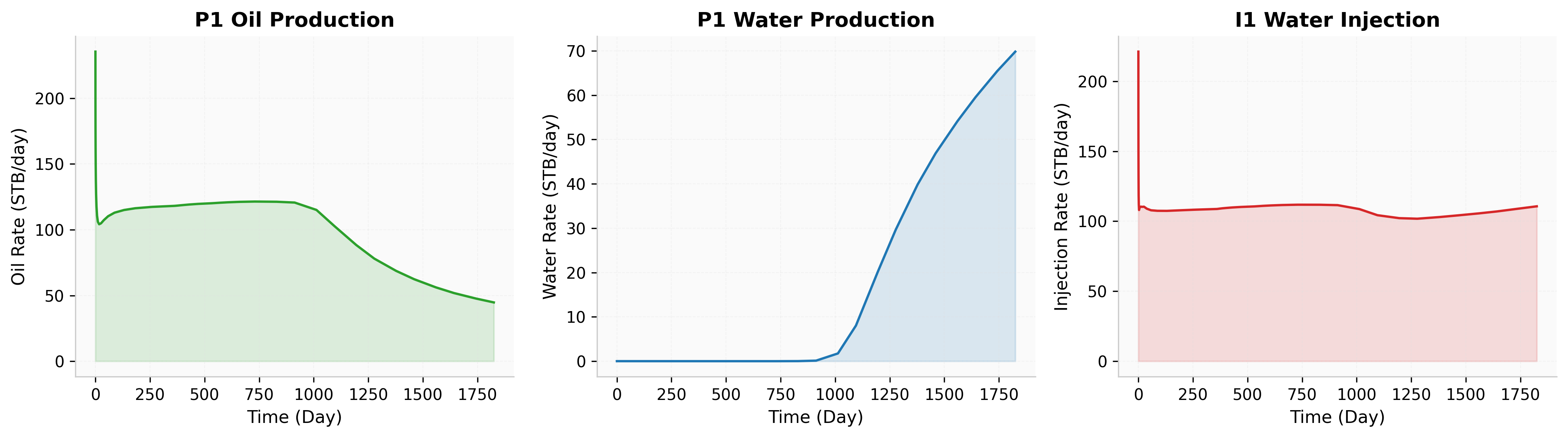
Fig. 63 Full simulation production curves.#
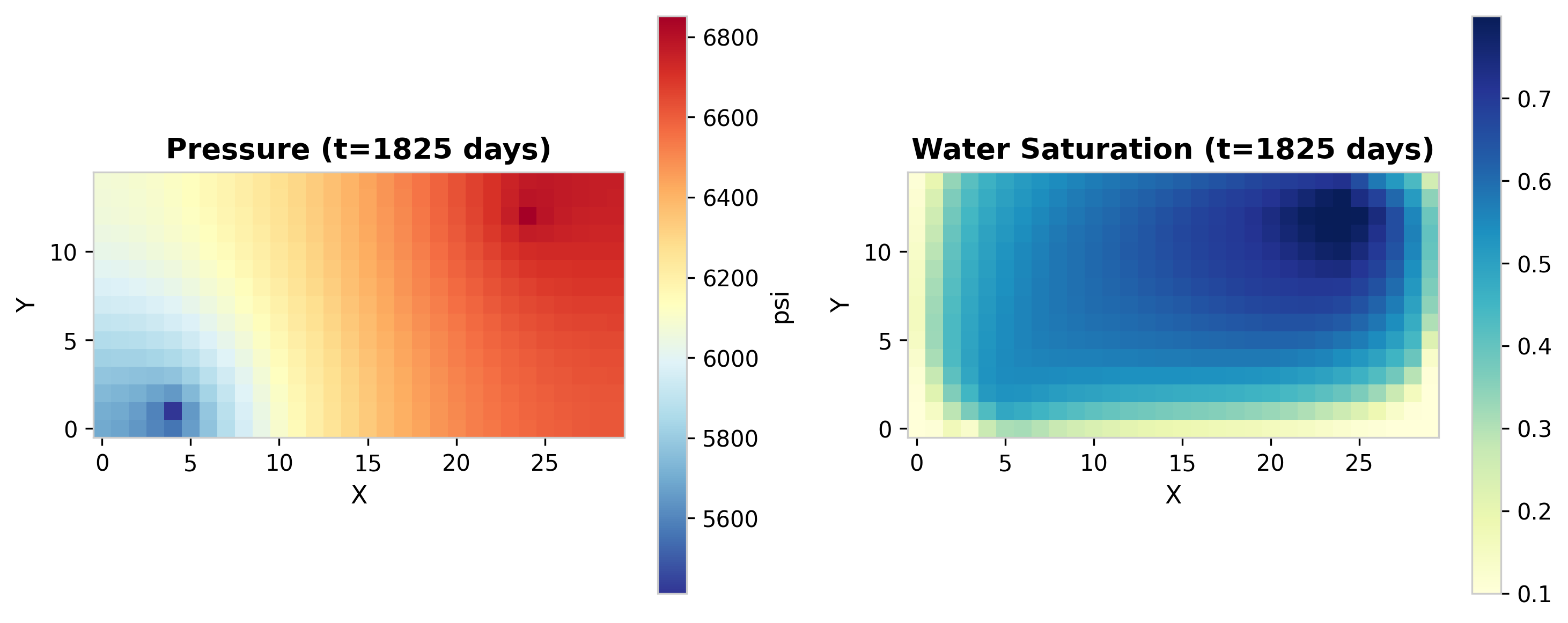
Fig. 64 Full simulation state maps: pressure and saturation.#
The step-by-step simulation reproduces the same results while allowing intermediate inspection. The snapshot below shows the reservoir state at t = 500 days.
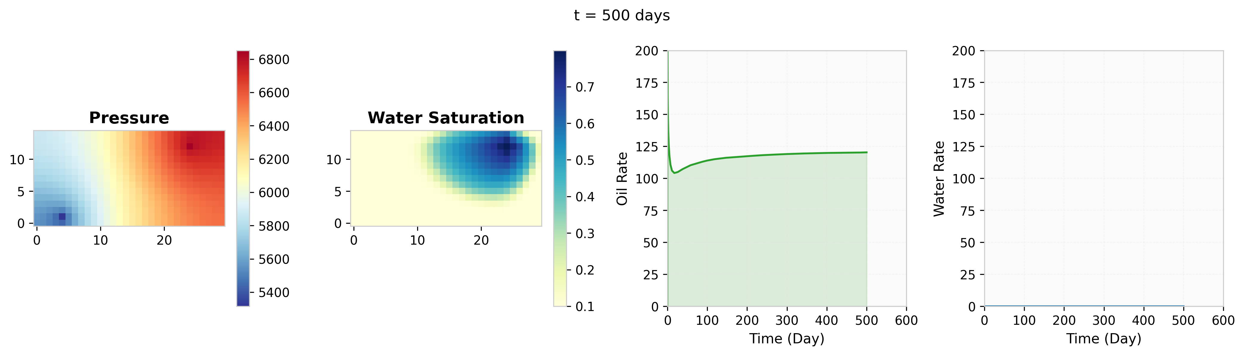
Fig. 65 Step-by-step simulation at t=500 days.#
When dynamic well operations are introduced – shutting in the original producer and opening a new well at a different location – the saturation front redirects toward the new producer, altering sweep efficiency.
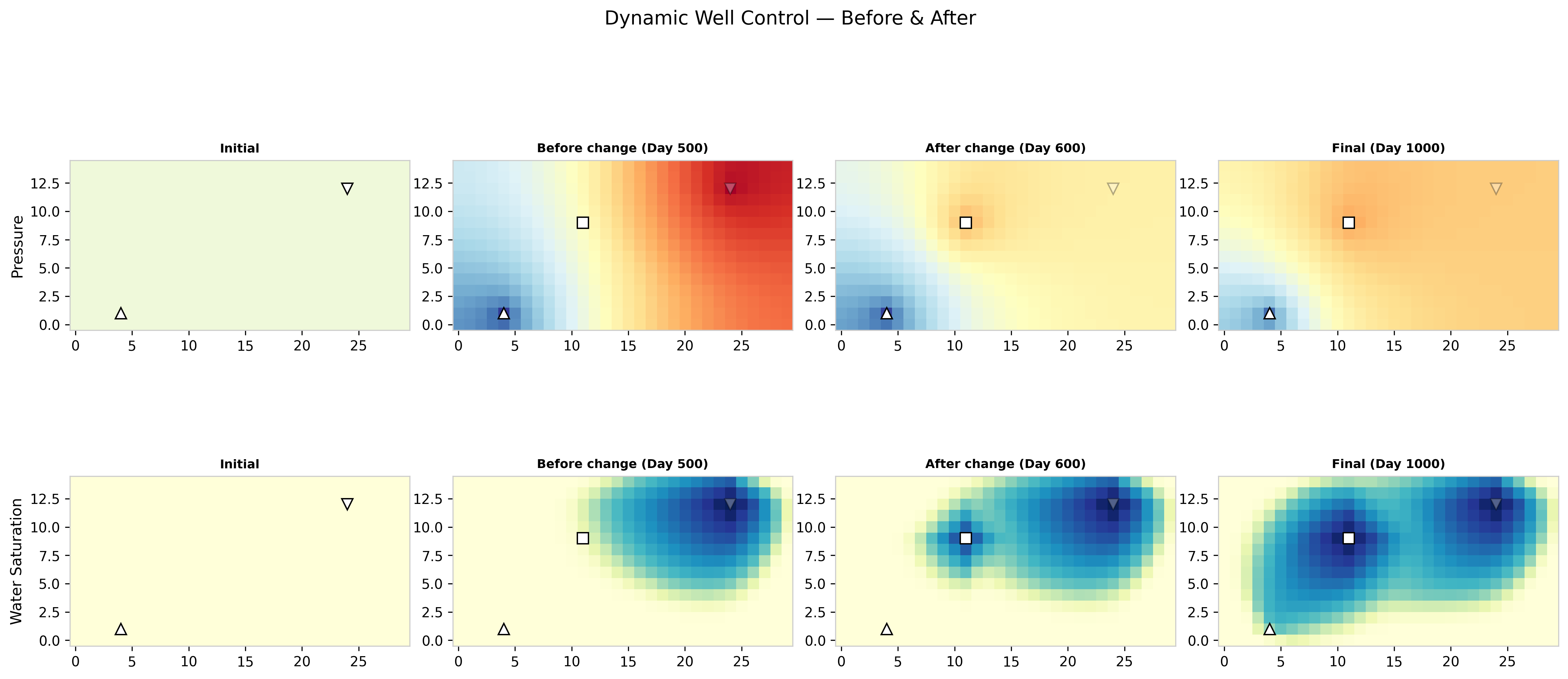
Fig. 66 Dynamic well control: saturation snapshots.#
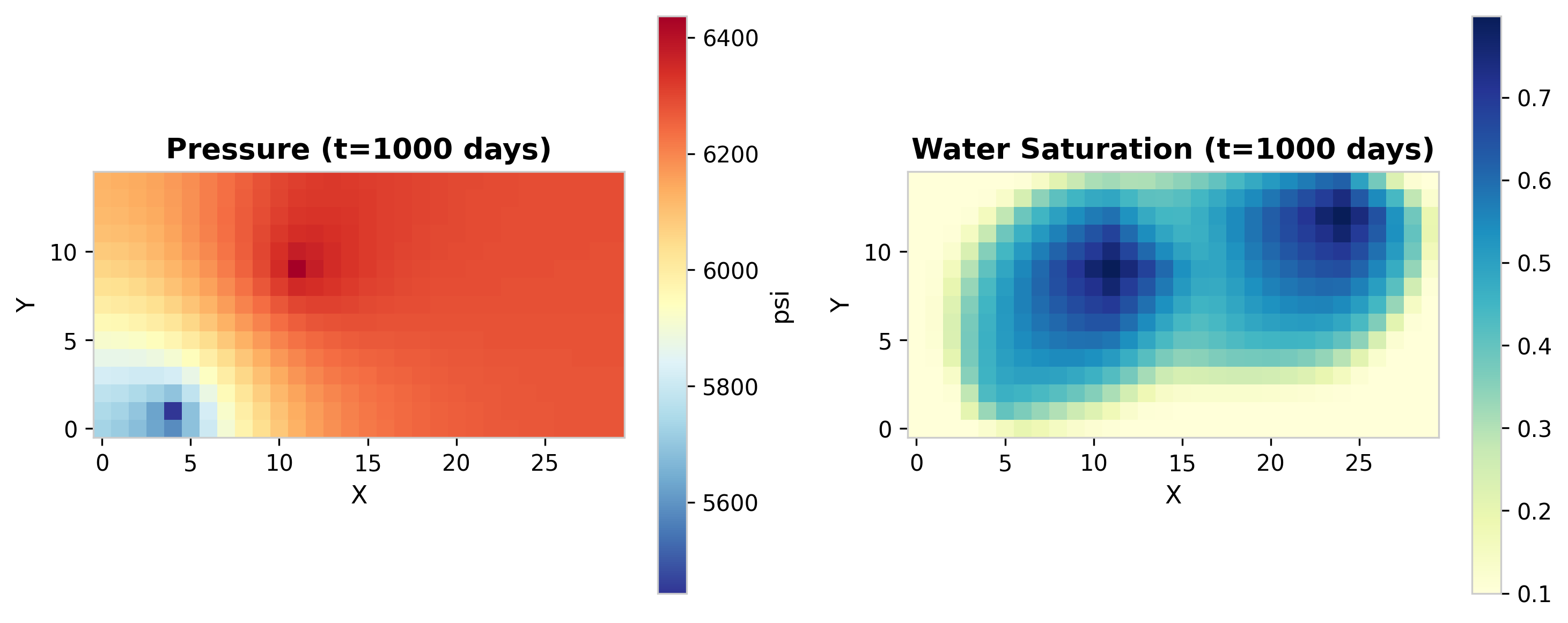
Fig. 67 Final state after dynamic well operations.#