Tutorial 09: Acoustic Full Waveform Inversion#
Note
This tutorial is available as a Python script examples/09_acoustic_fwi.py and an interactive Jupyter notebook examples/notebooks/09_acoustic_fwi.ipynb.
Recover the Marmousi2 velocity model from seismic data using gradient-based Full Waveform Inversion (FWI) with PyTorch automatic differentiation.
What You Will Learn#
Generate observed seismic data from a true velocity model
Start inversion from a smoothed initial model
Iterate the forward-misfit-backward-update loop
Monitor convergence and compare inverted vs. true models
Key Concepts#
Full Waveform Inversion (FWI) iteratively updates the velocity model to minimize the waveform misfit between simulated and observed seismic data. GeoBrain’s differentiable acoustic propagator provides exact gradients via automatic differentiation, avoiding the need for an adjoint-state implementation.
The inversion begins from a smoothed version of the true velocity model, which provides a low-frequency starting point that avoids cycle-skipping. At each iteration the forward solver generates synthetic shot gathers, the L2 waveform misfit is computed against the observed data, and PyTorch’s autograd back-propagates through the time-stepping loop to obtain the gradient with respect to every velocity cell. A simple gradient-descent update (or Adam optimizer) then nudges the model toward the true solution.
Code#
from geobrain.physics.wave import (
    AcousticModel, AcousticPropagator, GridConfig, BoundaryConfig,
)

# Enable gradient on velocity
model = AcousticModel(
    grid=grid, boundary=boundary,
    vp=vp_init, rho=rho,
    vp_grad=True,
    device='cuda',
)

propagator = AcousticPropagator(model, survey, device='cuda')

for epoch in range(n_epochs):
    result = propagator.forward(checkpoint_segments=4)
    loss = ((result['p'] - d_obs) ** 2).sum()
    loss.backward()
    # Update vp with gradient descent
Results#
The smoothed initial model removes sharp interfaces from the true Marmousi2 velocity field while retaining the large-scale trend, giving the optimizer a physically reasonable starting point.
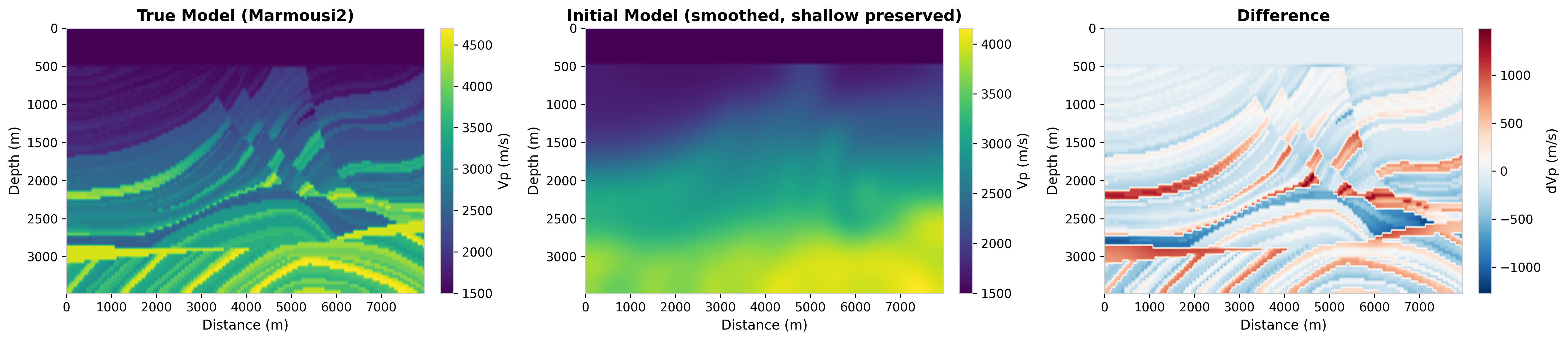
Fig. 58 Smoothed initial velocity model for FWI.#
After several hundred iterations the inverted model recovers the major structural features and velocity contrasts present in the true model.
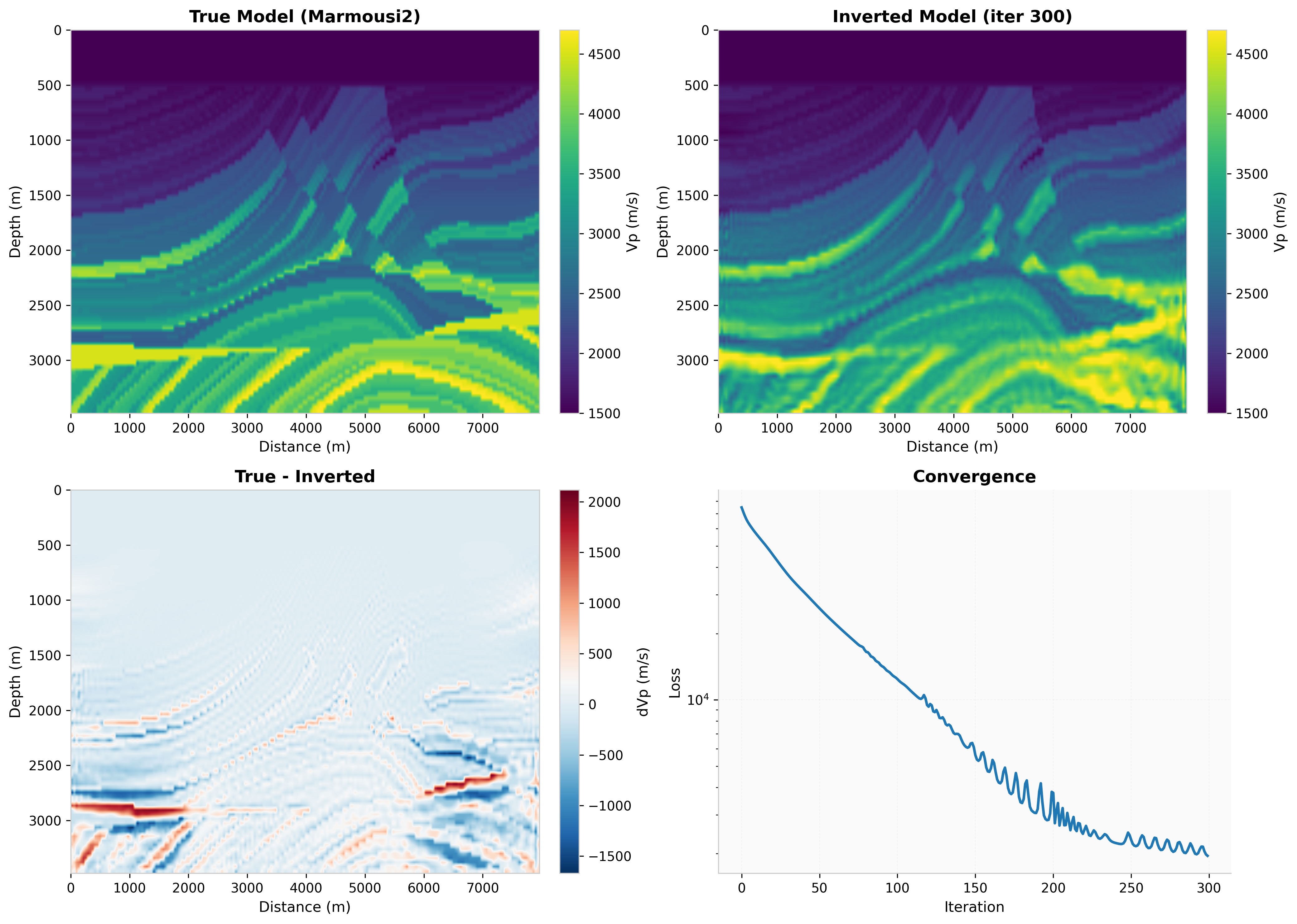
Fig. 59 FWI results: true model, initial model, and inverted model comparison.#