Tutorial 07: Acoustic Wave Propagation#
Note
This tutorial is available as a Python script examples/07_acoustic_forward.py and an interactive Jupyter notebook examples/notebooks/07_acoustic_forward.ipynb.
Run 2D acoustic wave simulations on the Marmousi2 model using the finite-difference time-domain (FDTD) solver with PML absorbing boundaries.
What You Will Learn#
Set up
GridConfigandBoundaryConfigBuild
AcousticModelwith velocity and densityConfigure
Source,Receiver, andSurveyRun
AcousticPropagatorwith gradient checkpointingVisualize shot gathers and wavefield snapshots
Code#
from geobrain.physics.wave import (
    GridConfig, BoundaryConfig, AcousticModel,
    Source, Receiver, Survey, AcousticPropagator,
    RickerWavelet,
)

grid = GridConfig(nx=200, nz=88, dx=40.0, dz=40.0)
boundary = BoundaryConfig(type='pml', n_layers=30, free_surface=True)
model = AcousticModel(grid=grid, boundary=boundary, vp=vp, rho=rho)

# Survey setup
source = Source(nt=NT, dt=DT, f0=5.0)
source.add_source(x=100, z=1, wavelet=wavelet_np)
receiver = Receiver(nt=NT, dt=DT)
receiver.add_receivers(x=rcv_x, z=rcv_z, receiver_type='pr')
survey = Survey(source, receiver)

# Forward modeling
propagator = AcousticPropagator(model, survey, device='cuda')
result = propagator.forward(checkpoint_segments=4)
Results#
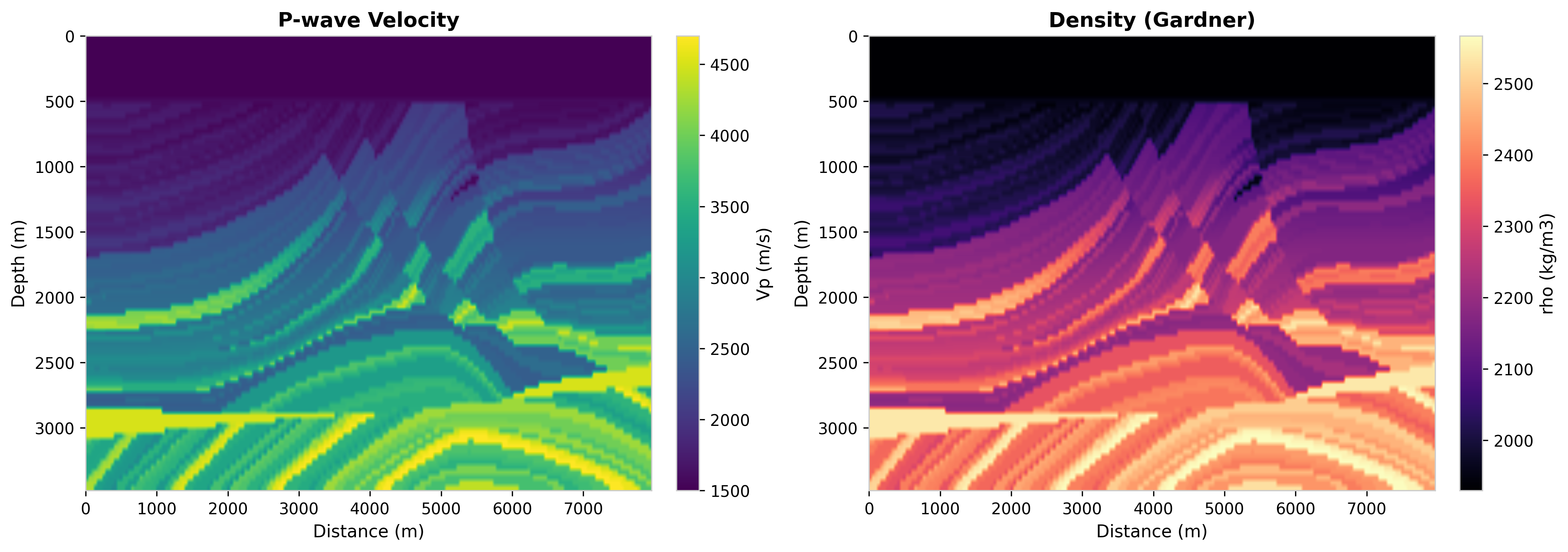
Fig. 49 Marmousi2 velocity and density model.#
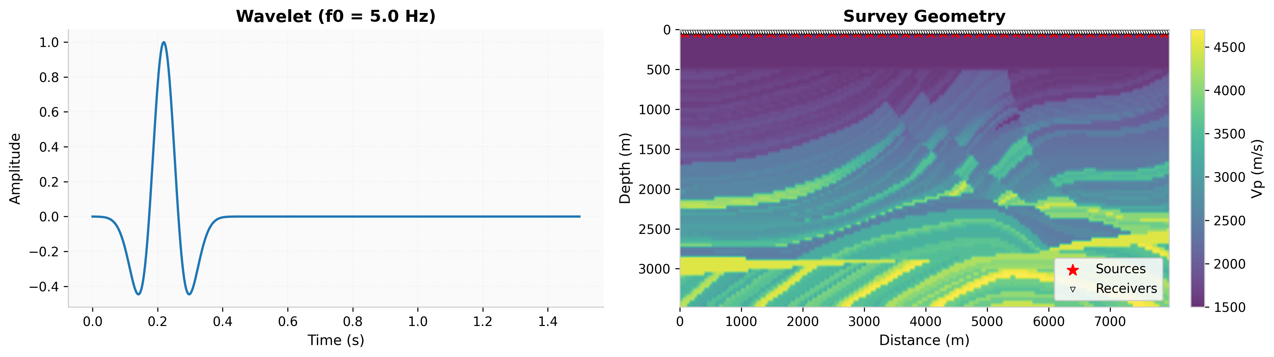
Fig. 50 Survey geometry: sources and receivers.#
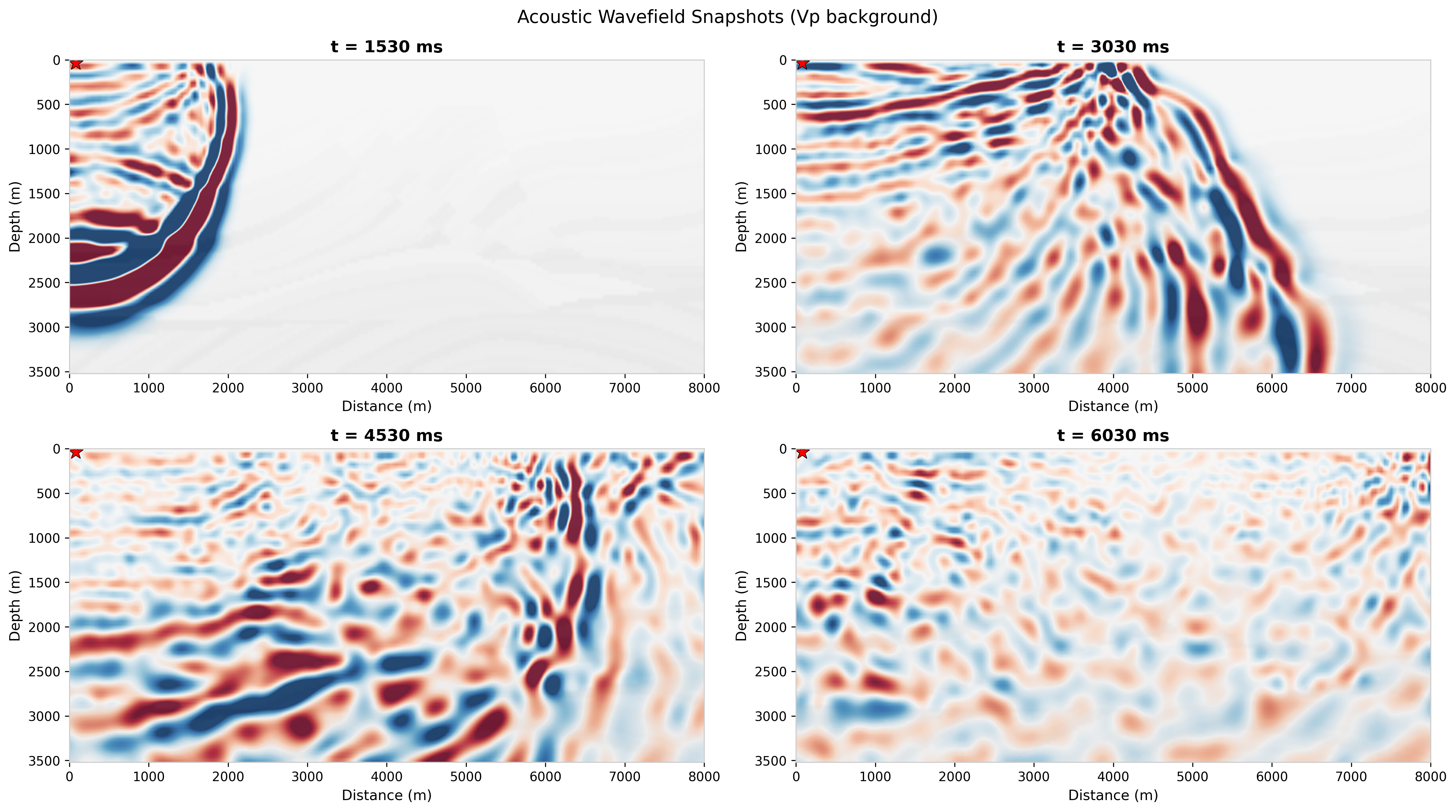
Fig. 51 Acoustic wavefield snapshots at different time steps.#
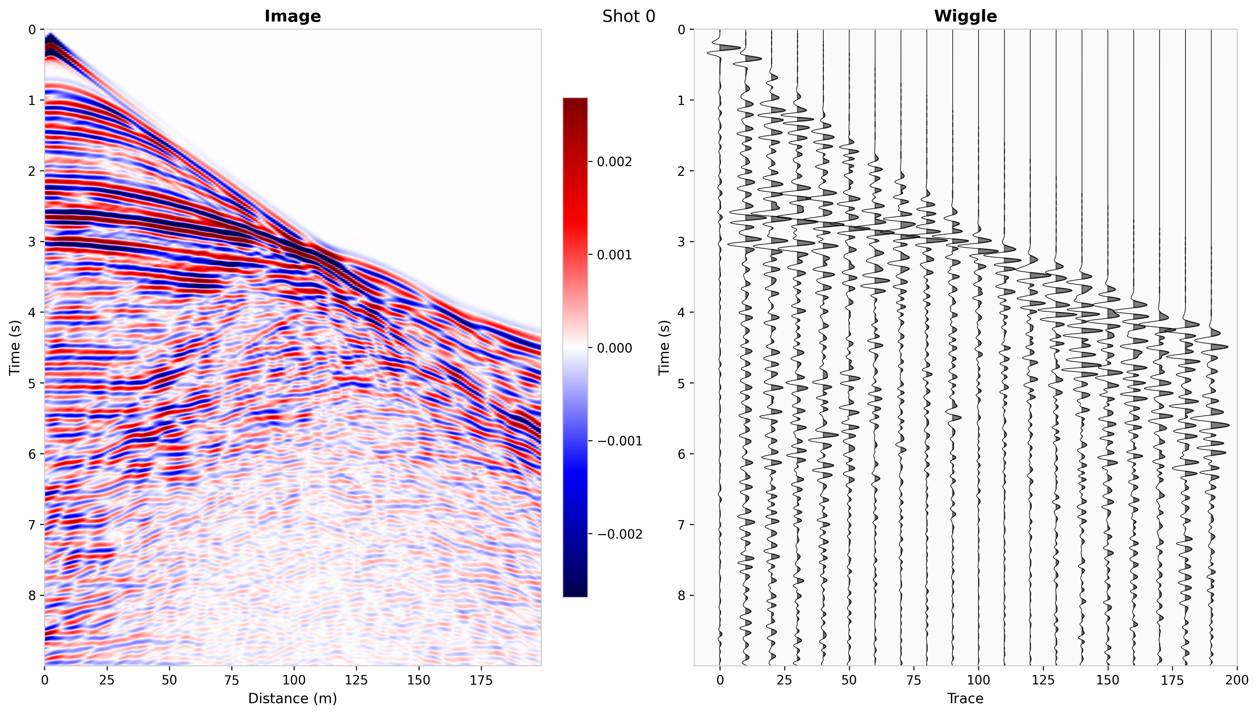
Fig. 52 Shot gather at the center of the model.#