Tutorial 08: Elastic Wave Propagation

Note

This tutorial is available as a Python script examples/08_elastic_forward.py and an interactive Jupyter notebook examples/notebooks/08_elastic_forward.ipynb.

Run 2D elastic wave simulations on the Marmousi2 model using the finite-difference time-domain (FDTD) solver with PML absorbing boundaries.

What You Will Learn

• Build IsotropicElasticModel with Vp, Vs, and density

• Configure PML boundaries with free surface

• Run ElasticPropagator and extract multi-component seismograms (P, Vx, Vz)

• Compare acoustic vs. elastic simulations on the same model

• Visualize wavefield energy and snapshot animations

Key Concepts

Elastic modeling captures both P-wave and S-wave propagation, including mode conversions at interfaces. Compared to the acoustic approximation, elastic modeling reveals S-wave arrivals and converted phases that carry additional information about lithology and fluid content.

Code

from geobrain.physics.wave import (
    GridConfig, BoundaryConfig, IsotropicElasticModel,
    Source, Receiver, Survey, ElasticPropagator, RickerWavelet,
)

grid = GridConfig(nx=200, nz=88, dx=40.0, dz=40.0)
boundary = BoundaryConfig(type='pml', n_layers=30, free_surface=True)

model = IsotropicElasticModel(
    grid=grid, boundary=boundary,
    vp=vp, vs=vs, rho=rho,
    device='cuda',
)

propagator = ElasticPropagator(model, survey, device='cuda')
result = propagator.forward(checkpoint_segments=4)

# Multi-component output
p_data = result.p       # Pressure
vx_data = result.vx     # Horizontal velocity
vz_data = result.vz     # Vertical velocity

Results

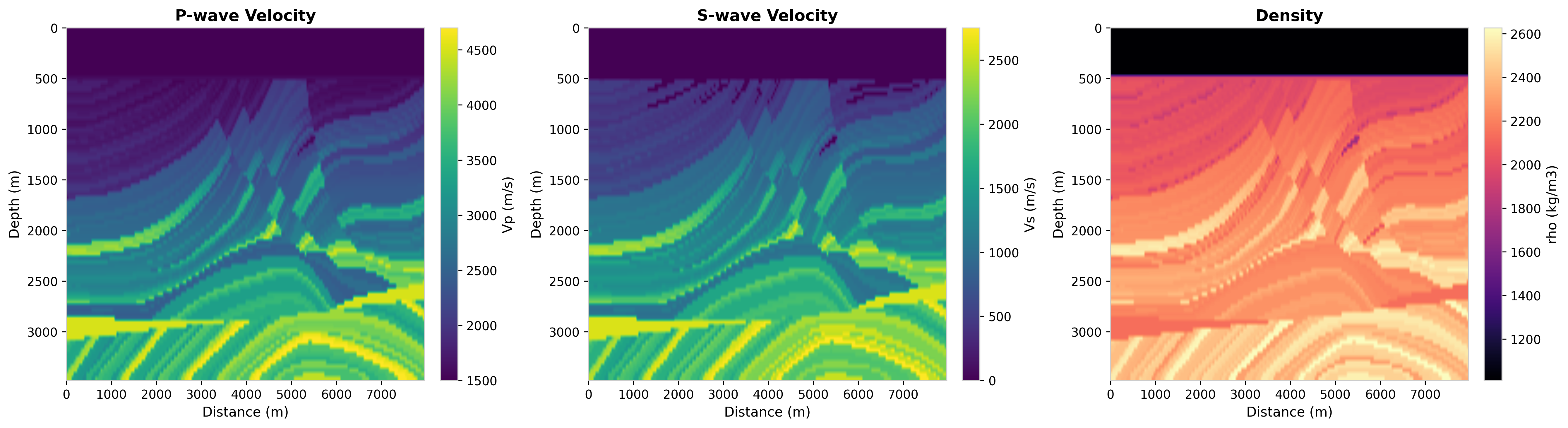
Fig. 53 Marmousi2 elastic model: Vp, Vs, density.

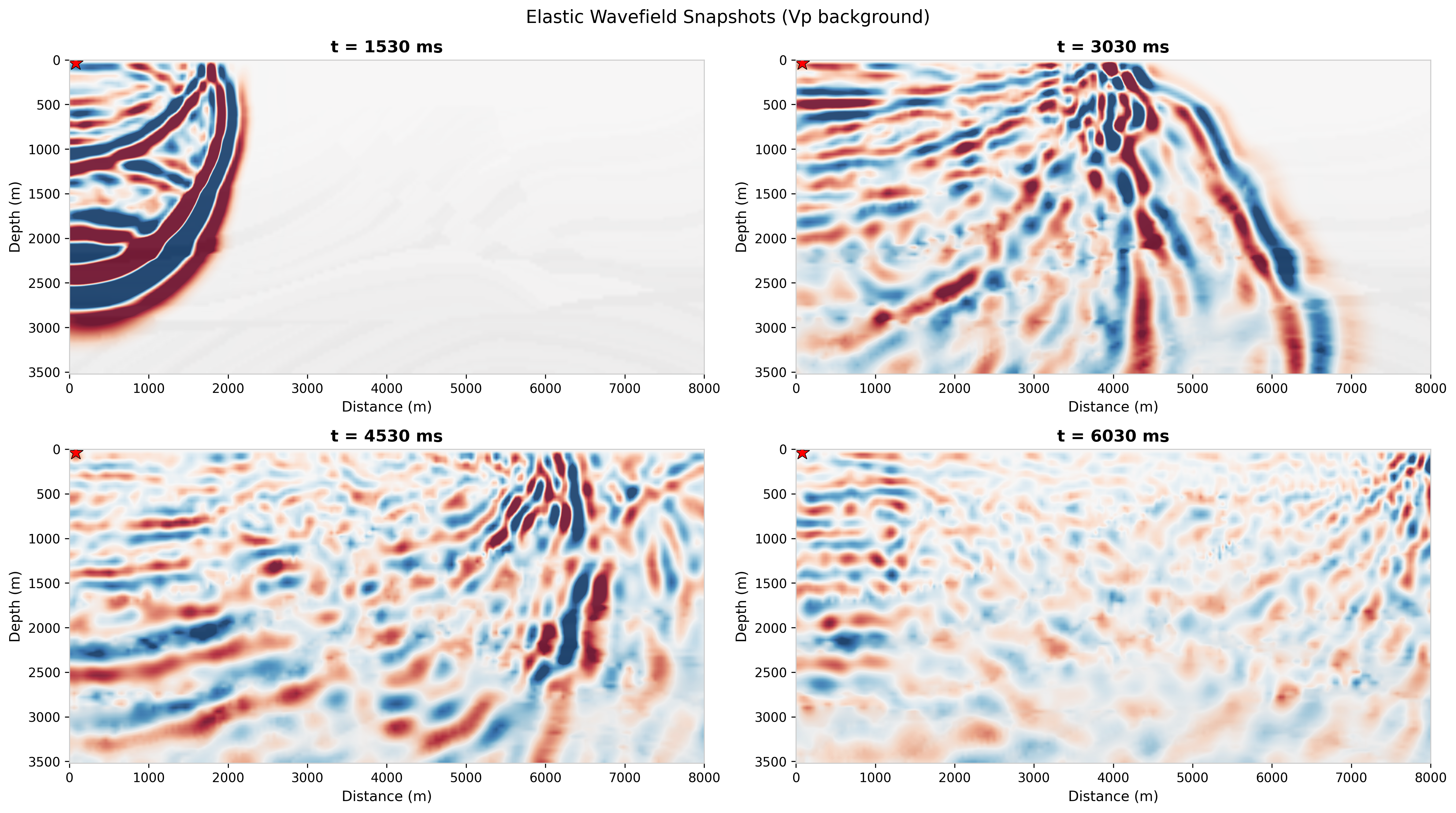
Fig. 54 Elastic wavefield snapshots showing P and S waves.

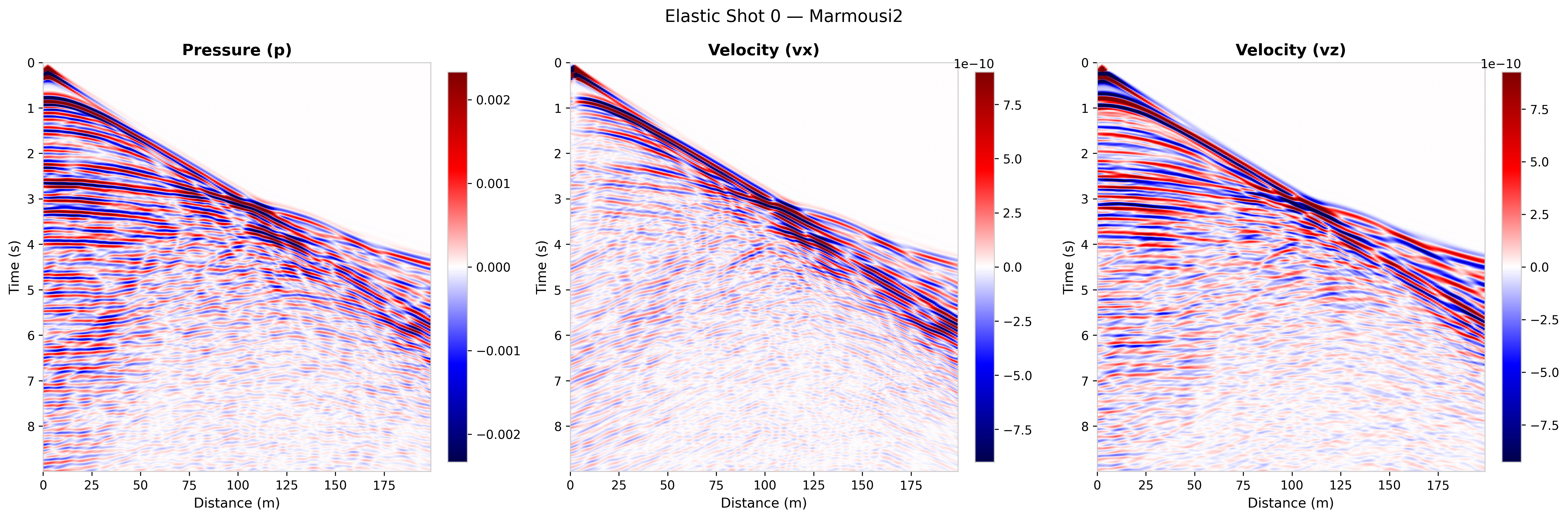
Fig. 55 Elastic shot gather: pressure, Vx, Vz components.

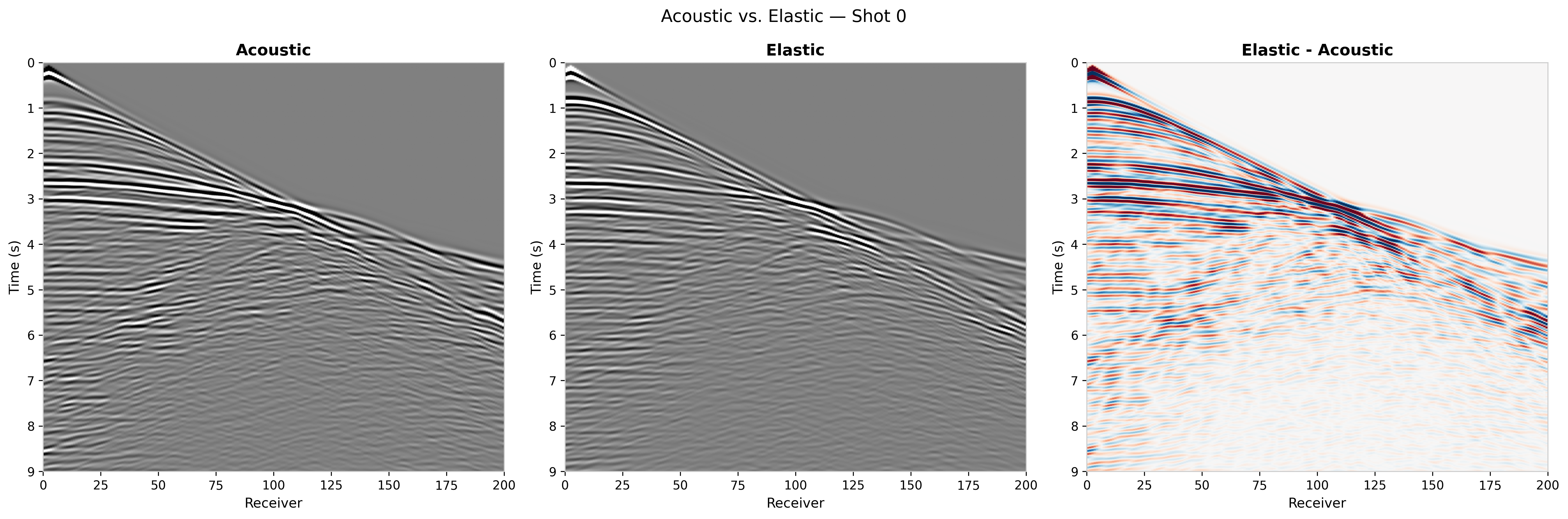
Fig. 56 Acoustic vs. elastic simulation comparison.

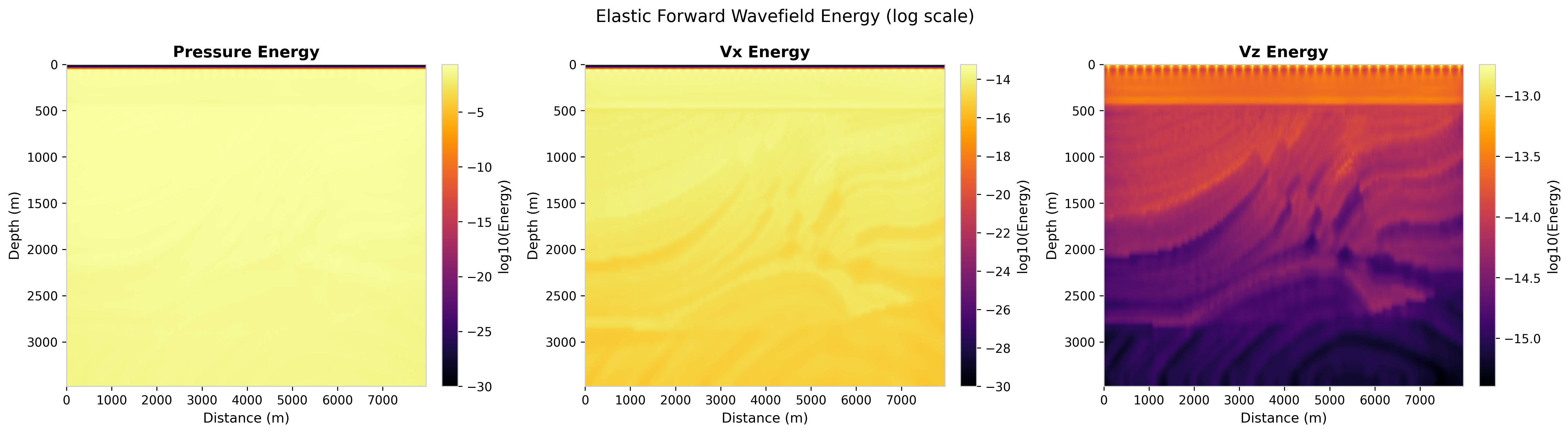
Fig. 57 Wavefield energy evolution over time.

Full Example

See examples/08_elastic_forward.py.