I/O and visualization (geobrain.io, geobrain.vis)

Getting data in and results out

Format	Read	Write
SEG-Y	read_segy → SegYData	write_segy
LAS well logs	read_las → LASData	n/a
EDI magnetotellurics	read_edi → EDIData	n/a
UBC mesh / model	read_ubc_mesh, read_ubc_model	write_ubc_mesh, write_ubc_model
HDF5	read_hdf5 → HDF5Data	write_hdf5
VTK	n/a	write_tensormesh_vtk, write_unstructured_vtk, write_points_vtk, write_octree_points_vtk

tensor_mesh_to_ubc_mesh and ubc_mesh_to_tensor_mesh convert between the UBC convention and GeoBrain’s; mesh_to_pyvista hands a mesh to PyVista for 3-D work. apparent_resistivity_ohm_m and impedance_phase_rad turn MT impedances into the quantities people actually plot.

Artifacts (save_tensor_artifact, save_npz_artifact, save_json_artifact and their loaders, with ArtifactRef) are for checkpointing an inversion or handing a result to the next stage.

Plotting (geobrain.vis)

Kind	Functions
2-D fields	plot_field_2d, plot_field_slice, plot_field_scatter, plot_field_tripcolor, plot_field_polygon
Meshes	plot_mesh_2d, plot_mesh_triangles, plot_mesh_quadtree
Inversion	plot_convergence, plot_comparison, plot_difference, plot_model_evolution, plot_sensitivity, plot_doi
Maps	plot_anomaly_map, plot_station_map
3-D	Scene3D, Slicer, view_volume, view_slices, view_isosurface, view_octree, view_points, view_survey, view_geomodel, view_reservoir, view_timelapse

Geometry

Every 2-D panel is drawn on node lines, and dx / dz say where those lines fall. A single number is a uniform grid. A graded grid has to hand over the widths themselves, either per cell or through the mesh:

import matplotlib
matplotlib.use("Agg")
import torch
from geobrain.mesh import TensorMesh
from geobrain.vis import plot_field_2d

mesh = TensorMesh(shape=(8, 12),
                  cell_widths=[torch.tensor([10.0] * 4 + [40.0] * 4),
                               torch.tensor([25.0] * 12)])
field = torch.zeros(8, 12)
field[4:] = 1.0

ax = plot_field_2d(field, mesh=mesh)
edges = sorted({round(float(v), 1) for v in ax.collections[0].get_coordinates()[:, 0, 1]})
print(edges)

[0.0, 10.0, 20.0, 30.0, 40.0, 80.0, 120.0, 160.0, 200.0]

Averaging those widths into one dz would put the contrast at 100 m instead of 40 m, so the mesh is not a convenience here. plot_field_2d, plot_field_slice, plot_comparison, plot_difference, plot_model_evolution, plot_sensitivity and plot_doi all accept it, and all accept a sequence of per-cell widths in dx / dz when there is no mesh object to hand. A mesh with no node lines, such as an unstructured one, is refused rather than approximated; plot those with plot_field_tripcolor or plot_field_polygon.

Physics-specific plotters

geobrain.vis holds what every sub-discipline shares. Plotters that only one family needs live in submodules and are imported from there, so the top-level namespace stays the cross-domain one:

Import from	Functions
geobrain.vis.seismic	plot_velocity_model, plot_gather, plot_section, plot_wavefield
geobrain.vis.em	plot_pseudosection
geobrain.vis.flow	plot_reservoir_state, plot_well_rates
geobrain.vis.geomodel	plot_geotable_2d

from geobrain.vis.seismic import plot_gather, plot_velocity_model

These are the ones that carry a domain default: plot_velocity_model opens on geo_velocity and plot_wavefield on geo_seismic, because a reader of those two pictures expects the convention before they expect anything else.

Colormaps

register_colormaps() registers the domain ramps, and get_colormap fetches one by name:

import matplotlib.pyplot as plt
from geobrain.vis import GEO_COLORMAPS, register_colormaps

register_colormaps()
print(sorted(GEO_COLORMAPS))
print("registered:", "geo_velocity" in plt.colormaps())

['geo_density', 'geo_porosity', 'geo_resistivity', 'geo_seismic', 'geo_velocity']
registered: True

Three of those exist because the domain convention is older than the argument about perceptual uniformity: a seismic amplitude is blue-white-red about zero (geo_seismic, which is a proper diverging ramp and simply correct), a velocity model is the cool-to-warm rainbow, and a resistivity section is the resistivity rainbow. The examples gallery uses all three, and says in its own README why it uses rainbows there and perceptually uniform ramps everywhere else.

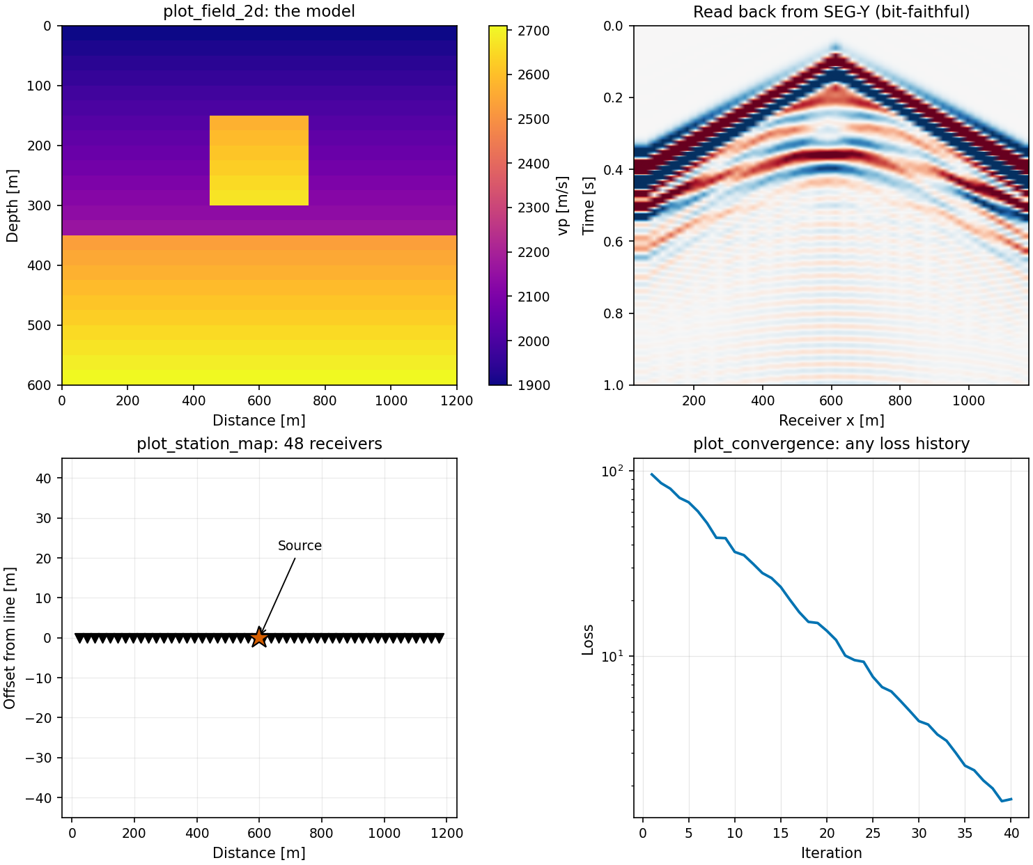
SEG-Y, VTK and HDF5 in, geobrain.vis out. From examples/01_architecture/08_data_io_and_figures.py.

See also

• examples/01_architecture/08_data_io_and_figures.py: SEG-Y, VTK and HDF5 in, geobrain.vis out.

• examples/README.md covers the figure conventions the gallery holds to.