Electromagnetics (geobrain.physics.em)

The electromagnetic family, galvanic through inductive, in one module.

Method	Operators
DC resistivity	DC2D, DC25D, DC3D
Induced polarization	IP2D, IP3D, IPSimulator, IPChargeabilityModel
Spectral IP	SIP, SIPColeColeModel
Magnetotellurics	MT1D, MT2D, MT3D
Frequency-domain EM	FDEM3D, FDEMCyl, HEM, VTEM
Time-domain EM	TEM1D, TEM3D, WaveformTEM1D
Controlled source	CSEM1D
Self potential	SelfPotential2D

Each has its own survey type (DC2DSurvey, MT1DSurvey, FDEM3DSurvey, TEM1DSurvey and the rest), and the electrode, loop or station geometry lives there rather than in the operator, so one operator serves many acquisitions. DipoleDipoleSurvey and BoundDipoleDipoleSurvey build the standard arrays.

Conductivity, Resistivity, Permittivity and Permeability wrap the physical properties; ComplexData, FieldComponent and TimeWaveform describe what comes back.

Before you run one

Topography is not decoration. The standard treatment is to let the mesh continue above the ground, give the cells above the surface the conductivity of air, and drape the electrodes onto the first ground cell in each column. Nothing about the operator changes: the air is just very resistive rock. But the air cells must be held fixed during inversion: their gradient is the largest in the model, because a tiny conductivity in the denominator makes the objective extremely sensitive there, and inverting them fills the sky with current.

Apparent chargeability is a ratio of two solves. It is (V_eta - V_inf) / V_eta, so the dipole difference has to be taken on each potential separately, before the ratio is formed. Differencing apparent chargeability between receivers is not a thing you may do.

Chargeability is bounded. It lives in [0, 1), so it is inverted through a sigmoid rather than as a free parameter: an unbounded step drives the effective conductivity sigma_inf (1 - eta) negative and the solve fails. The starting model matters too. Start at eta = 0.2 everywhere and the optimizer sits there; start near zero and it finds the body.

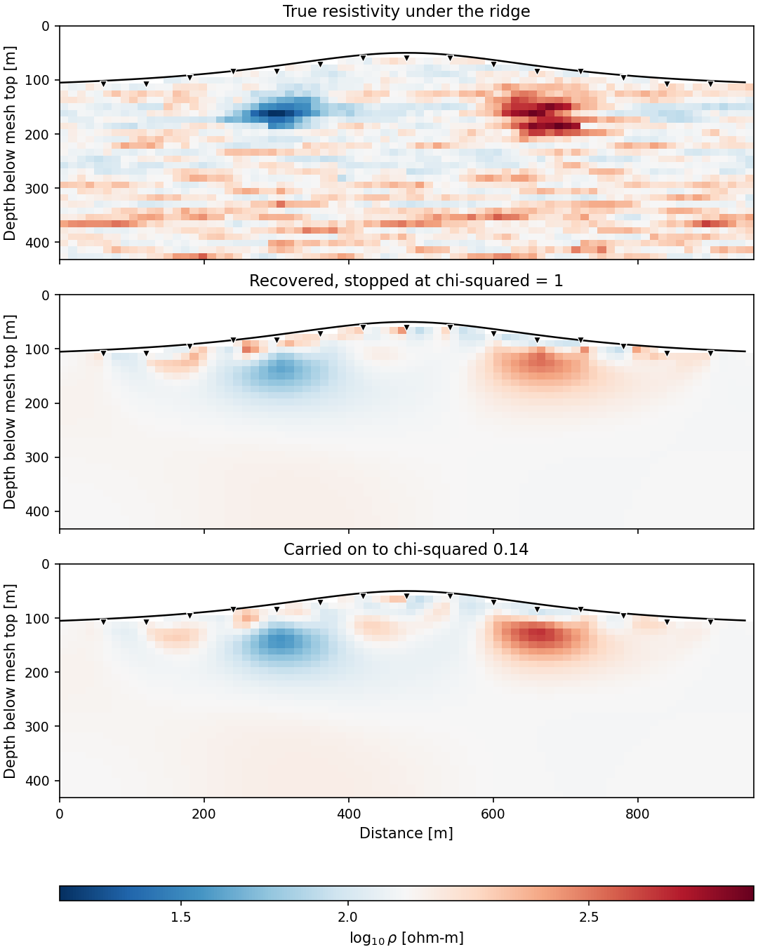
A DC survey over topography, inverted until chi-squared reaches 1. From examples/03_physics/02_dc_resistivity.py.

Stopping

Data carry noise, so a model that drives the misfit to zero is fitting noise and will grow structure to do it. The EM examples watch chi-squared, the misfit in units of the noise, and stop at 1, which is the statistically honest place to stop, and it is a rule rather than an iteration count.

See also

• examples/03_physics/02_dc_resistivity.py: a survey over a ridge, and chi-squared as the stopping rule.

• examples/03_physics/03_induced_polarization.py: the image resistivity cannot give you.

• examples/03_physics/05_em_induction.py: one airborne sounding, four decades of frequency, a layered earth read back out.